User Guide
Welcome to the AMIGOpy User Guide. This section will walk you through the core workflows of loading data, navigating the interface, and performing image analysis.
Loading Data
AMIGOpy provides several flexible methods to load your medical images, 3D structures, dose distributions, and CAD/3D printing models.
Method 1: Windows Explorer Integration (Recommended)
You can launch AMIGOpy and load entire datasets directly from Windows Explorer:
* Loading a Folder: Right-click any folder containing your dataset in Windows Explorer, select Open with, and choose AMIGOpy. AMIGOpy will launch and automatically scan and load all files recursively inside that folder.
* Loading Individual or Grouped Files: Select a single .dcm (DICOM) file, or select a group of files, right-click, select Open with, and choose AMIGOpy.
Method 2: Drag and Drop With the AMIGOpy interface already open, you can drag and drop folders or individual files directly from Windows Explorer into the Data Tree panel on the left side of the window to load them.
Method 3: Top Navigation Menu You can open files from the top menu by going to File ➔ Open and selecting your desired format.
AMIGOpy supports various keyboard shortcuts to open standard formats:
* DICOM (Ctrl + D) — Select a folder, and AMIGOpy will recursively load all DICOM slices, RTDoses, RTStructs, and RTPlans inside.
* NIfTI (Ctrl + N) — Open NIfTI volumetric data (.nii, .nii.gz).
* AMIGOpy (Ctrl + A) — Open native workspace files.
* IrIS (Ctrl + I) — Open IrIS formats.
Navigating the Interface
Once your data is loaded, the interface displays the volumetric views and analysis panels:
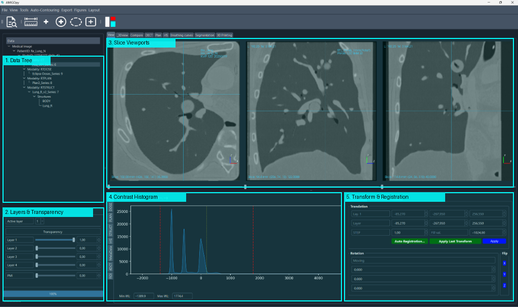 Figure 1: The AMIGOpy main interface layout, with numbered annotations matching the panels below.
1. Data Tree (Left Panel)
All loaded items are organized in the hierarchical Data Tree menu on the left side (marked as 1 on the interface diagram):
* Grouped by format (e.g., Medical Image ➔ DICOM).
* Organized by PatientID, StudyID, Modality (e.g., CT, RTDOSE, RTSTRUCT, RTPLAN), and Series.
* Under RTSTRUCT, you can expand and view individual contoured structures (e.g., BODY, Lung_R).
2. Layers & Transparency Panel (Bottom-Left) Located directly below the Data Tree (marked as 2 on the interface diagram): * Controls active visualization layers (supporting up to 4 concurrent image layers). * Individual transparency sliders to blend slices and structures seamlessly.
3. Slice Viewports (Top Panels) The main display features three orthogonal slice rendering viewports (marked as 3 on the interface diagram): * Axial view (Transverse) — left pane. * Sagittal view — middle pane. * Coronal view — right pane. Each view contains position lines indicating cross-sectional alignment and slider controls below the viewports to page through slices.
4. Contrast Histogram (Bottom-Center Panel) The histogram panel at the bottom center plots the distribution of Hounsfield Units (HU) or voxel intensities in the loaded scan (marked as 4 on the interface diagram): * The graph helps visualize the image contrast. * The red vertical dotted lines indicate the current window boundaries. * You can adjust the Min WL and Max WL values using the text inputs below the plot to adjust contrast windowing manually.
5. Transform & Registration Panel (Bottom-Right) Located at the bottom right corner (marked as 5 on the interface diagram): * Translation and rotation inputs to manual align scans. * Auto Registration trigger buttons (for intensity-based mutual alignment of multiple datasets).
Mouse Controls in Slice Views
Interact with the viewports using your mouse: * Window & Level: Left-click and hold inside any slice view, then drag the mouse to dynamically adjust the contrast Window (width) and Level (center). * Zooming: Right-click and hold, then drag up/down to zoom in or out on the slice. * Panning (Dragging): Click and hold the mouse wheel (middle click), then drag the mouse to pan the image around the viewport.